Measuring audio signals accurately forms the backbone of any reliable visual performance system. A well tuned audio pipeline breaks a raw stereo mix down into distinct control signals that drive video parameters in real time. By separating bass frequencies from high hats, identifying fast transients, and mapping the dynamic range of a live input, you link sound directly to motion on the screen behind you.
The Audio Analysis Engine Architecture
Every sound that reaches a device must be converted into numerical data before it can manipulate a video layer. The core of this system operates on a continuous stream of audio samples processed in discrete blocks.
The engine uses a 512-sample hop size within an AudioWorklet pipeline to balance temporal precision with computational efficiency. 6 milliseconds of audio.
This specific duration provides enough resolution to capture fast percussive hits while keeping processing latency low enough for live visual synchronization. When the audio signal enters the pipeline, the engine performs a Fast Fourier shape.
This mathematical operation converts the time-domain waveform into a frequency-domain spectrum. The spectrum reveals the exact amplitude of individual frequency bins at that specific moment in time.
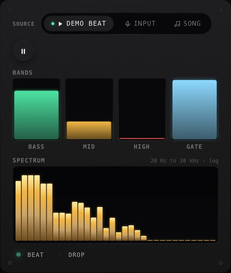
The engine then aggregates these bins into distinct frequency bands. Instead of treating the entire audio track as a single volume level, band splitting isolates specific musical elements.
You can target the low end, the midrange, and the high end separately. The separated signals are then conditioned using peak and Root Mean Square detection methods.
Peak detection tracks the absolute highest sample value within the current buffer. This method responds instantly to sharp spikes in audio energy.
You map peak signals to visual parameters that require rapid, jerky movements, such as the scale of a 3D object, the rotation speed of a camera, or the trigger for a strobe effect. Root Mean Square detection calculates the continuous average energy of the signal over time.
This approach smooths out the rough edges of the waveform. Root Mean Square signals provide a slow, gliding modulation source.
You map Root Mean Square signals to parameters like the opacity of a video clip, the intensity of a color shift, or the blur radius of a background layer. Balancing peak and Root Mean Square detection gives you precise control over the texture of your visual performance.
A drum and bass track requires tight, aggressive visual changes driven by peak detection on the kick and snare. An ambient set relies on Root Mean Square detection to slowly fade textures in and out as the synthesizer chords swell and decay.
By understanding the flow of data from the raw input buffer through the Fourier shape and into the smoothing algorithms, you gain the ability to dial in the exact response characteristics needed for your set. The entire pipeline runs on a dedicated audio thread.
This separation prevents the main user interface thread or the heavy graphics rendering thread from interrupting the audio analysis. If the device struggles to render a complex video shader, the audio thread continues to process incoming sound without dropping blocks.
The resulting parameter values are then passed across the thread boundary, ready to be read by the visual engine on the next render frame. This architecture guarantees that the audio analysis remains tight, predictable, and tightly coupled to the incoming beat.
Frequency Band Calibration: Bass, Mid and High
Breaking the audio spectrum into functional bands allows you to isolate specific instruments. A typical club mix contains a dense wall of sound.
If you map the master volume to a visual effect, the screen will flash randomly and erratically. By filtering the signal into bass, mid, and high bands, you extract meaningful musical information from the chaos.
The bass band typically covers frequencies from 20 Hz up to 250 Hz. This region contains the fundamental frequencies of kick drums, sub bass synthesizers, and bass guitars.
In electronic music genres, the bass band provides the rhythmic foundation. When you isolate the bass band, you isolate the pulse of the track.
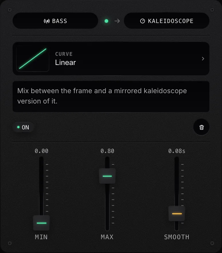
You route the bass signal to parameters that dictate the physical scale and impact of your visuals. A heavy kick drum hit can scale a 3D model up by a factor of two, push a video plane toward the camera, or trigger a full screen color inversion.
The mid band spans from 250 Hz to roughly 4000 Hz. This frequency range holds the majority of melodic and harmonic content.
Lead synthesizers, vocal lines, snare drum bodies, and rhythm guitars live in the mid band. The mid band often dictates the emotional arc of a song.
Because this band contains a wide variety of sounds, the resulting signal tends to be complex and sustained. You map the mid band to parameters that alter the texture or hue of your output.
As a synthesizer filter opens up and allows more high mid frequencies through, you can drive a parameter that shifts the color palette from cool blues to warm oranges. You can also map the mid band to the speed of a video clip, causing the playback to accelerate as the melodic intensity increases.
The high band covers the spectrum from 4000 Hz up to 20000 Hz. This region consists of sharp, transient rich sounds like hi-hats, cymbals, tambourines, and the airy sizzle of distortion.
High frequencies dictate the groove and momentum of a drum beat. The high band signal typically consists of rapid, short bursts of energy.
You route the high band to parameters that require fast, flickering responses. You can map it to the opacity of an overlay layer, causing a secondary texture to flash into existence on every sixteenth note hi-hat hit.
You can also use the high band to modulate the density of a point element system or the grain amount on a post processing effect.
| Frequency Band | Typical Range | Primary Instruments | Suggested Visual Mapping |
|---|---|---|---|
| Bass | 20 Hz - 250 Hz | Kick drums, 808s, sub bass | Scale, camera zoom, full screen flashes |
| Mid | 250 Hz - 4000 Hz | Vocals, synths, snare bodies | Color shifts, blur radius, playback speed |
| High | 4000 Hz - 20000 Hz | Hi-hats, cymbals, air, noise | Opacity flickers, point element density, grain |
Calibrating the exact crossover points between these bands is a critical step before a show. A techno track might require a lower bass crossover point to isolate a deep sub kick, while a house track might benefit from a slightly higher bass crossover to catch the punchy mid bass lines.
The engine allows you to adjust these cutoffs in real time. You monitor the visual output while turning the crossover dials until the video reaction perfectly matches the groove of the music.
Proper band calibration prevents overlapping signals. If your bass band spills into the mid range, your visual kick drum triggers will become muddy and loose.
Clean separation results in sharp, distinct visual events.
Transient Detection and Beat Tracking
Beyond simply measuring volume levels across frequency bands, advanced audio analysis involves identifying structural events within the music. Transient detection focuses on locating the exact moment a sound begins.
A transient is a short duration, high amplitude peak that occurs at the beginning of a waveform. When a drumstick strikes a snare drum, or a synthesizer envelope fires with a zero millisecond attack time, a transient is generated.
The detection algorithm monitors the incoming audio buffer for sudden increases in energy. Instead of looking at the absolute volume, the algorithm calculates the energy difference between the current block of 512 samples and the previous block.
When this energy delta exceeds a predefined threshold, the system registers a transient event. This method is highly effective for extracting drum hits from a complex mix, even if the overall volume of the track is already loud.
By isolating transients, you generate discrete trigger signals rather than continuous modulation signals. You map transient triggers to actions that happen instantly.
Instead of modulating a value smoothly over time, a transient trigger acts like a digital switch. You use it to swap the active video clip, advance a sequence of images, trigger a generative pattern to redraw, or fire a quick burst of white noise on the screen.
Because transients occur at the exact moment a note is played, the visual response feels incredibly tight and synchronized. Extracting specific types of transients requires combining onset detection with frequency band isolation.
To extract only the kick drum hits, you run the transient detection algorithm exclusively on the bass frequency band. The system ignores sharp snare hits or hi-hats because they exist in higher frequency ranges.
To extract the snare hits, you target a narrow slice of the mid frequency band. This precise extraction allows you to build complex visual rhythms.
You can route the kick drum transients to swap clips on layer one, and route the snare drum transients to invert the colors on layer two. Auto-gain calibration plays a vital role in keeping transient detection accurate throughout a performance.
In a live club environment, the overall volume of the music changes constantly. A DJ might push the master fader up during a heavy drop, or pull the bass equalizer down during a breakdown.
If the transient detection threshold remains fixed, the system will miss hits during quiet sections and generate false triggers during loud sections. The auto-gain system continuously measures the average loudness over a rolling window of several seconds.
It dynamically adjusts the internal input gain to keep the audio signal within the optimal range for the detection algorithm. This automatic leveling ensures that your visuals react consistently, regardless of how the DJ manipulates the mixing console.
Beat tracking takes transient detection one step further. While transient detection finds individual hits, beat tracking algorithms analyze the pattern of those hits over time to determine the underlying tempo.
The system estimates the current Beats Per Minute by measuring the time intervals between successive prominent transients. Once the system locks onto the tempo, it generates a continuous phase signal that ramps from zero to one over the duration of each beat.
This beat phase signal allows you to synchronize slow, cyclical visual animations to the grid of the music. You can map the beat phase to the rotation of a 3D camera, ensuring that it completes exactly one full revolution every four beats.
Noise Gate and Sensitivity Configuration
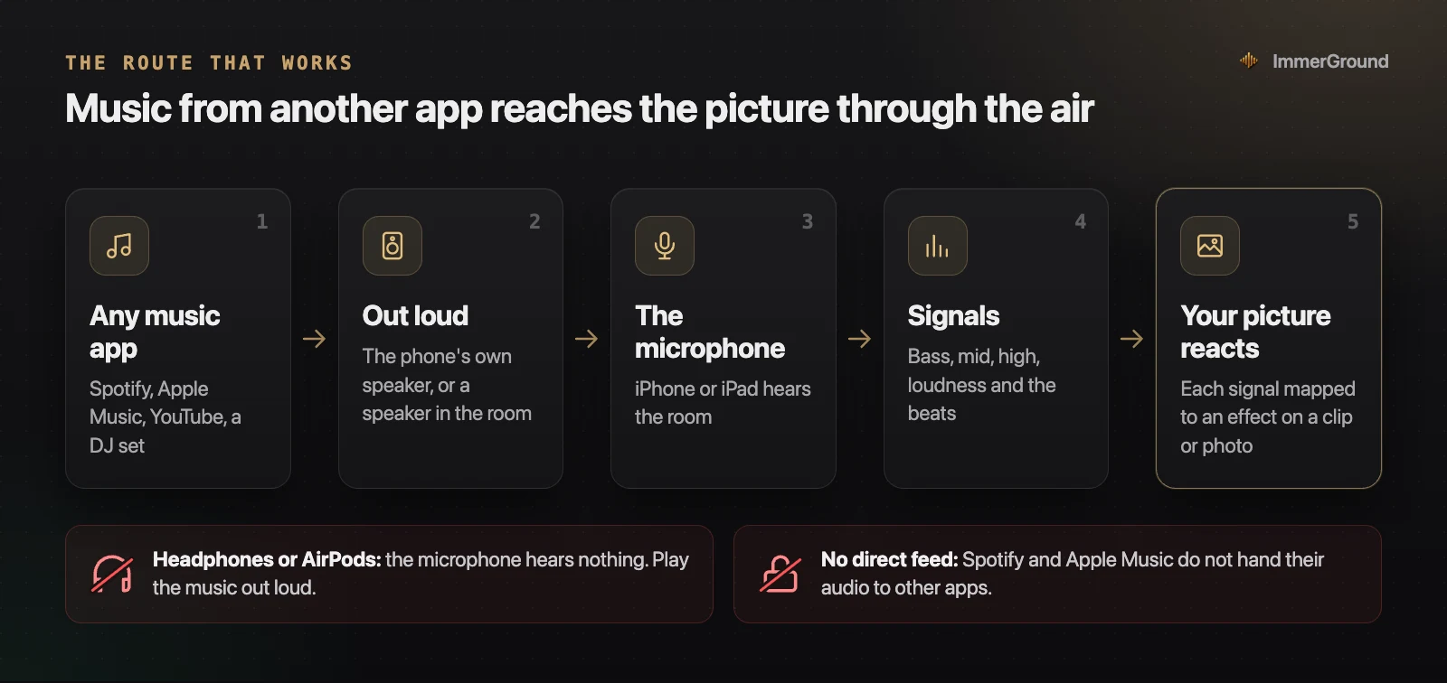
Handling live audio in a physical space introduces the challenge of background noise. If your microphone or line input picks up the hum of an air conditioner, the chatter of a crowd, or the mechanical vibration of a stage, your visuals will react to that noise.
To maintain a clean visual output, you must configure a noise gate. A noise gate acts as a barrier that blocks all audio signals below a specific volume threshold.
The system implements a hard cut at -54 dB by default. Any signal quieter than -54 dB is forced to absolute zero.
This prevents ambient room noise from registering in the analysis engine. The visual parameters remain perfectly still until a deliberate, loud musical element breaks through the gate threshold.
When the music stops entirely, the visuals snap to their idle state, rather than twitching nervously in response to the noise floor. You adjust the noise gate threshold based on your specific environment.
In a quiet recording studio, you might lower the gate to -70 dB to capture subtle reverb tails and quiet acoustic instruments. In a loud, echoing club environment where the crowd is shouting and the monitors are feeding back, you might need to raise the gate to -40 dB.
At this level, only the direct, percussive hits of the sound system will pass through the analysis pipeline. Ambient room isolation is critical when using a microphone instead of a direct line feed.
A microphone placed near the DJ booth will pick up the main PA system, but it will also capture reflections from the walls and ceiling. These reflections smear the transients and muddy the frequency bands.
A tight noise gate helps cut off the reverberant tails, leaving only the sharp initial attacks for the analysis engine to process. This technique sharpens the visual response significantly in poor acoustic environments.
Feedback loops pose a major threat when generating audio reactive visuals. If your visual system outputs an audio signal itself, and that audio signal is picked up by your analysis microphone, the system will trigger itself in an infinite loop.
The screen will lock up in a state of maximum intensity. The noise gate serves as the first line of defense against feedback, but proper routing is essential.
You must ensure that the audio generated by the visual device is not routed back into its own input channel. Sensitivity dials provide manual control over the dynamic range of the incoming signal after it passes the noise gate.
If the input source is weak, you increase the sensitivity. The engine applies a mathematical multiplier to the sample values, pushing them higher before they reach the frequency splitters.
If the input source is too hot and constantly hits the maximum value, all nuance is lost. The visual parameters will stay pegged at one hundred percent.
You decrease the sensitivity to pull the signal down, restoring the dynamic range and allowing the visuals to breathe. Proper gain staging requires setting the hardware input volume correctly on your audio interface first, then fine tuning the software sensitivity dials to map the signal perfectly to your visual parameters.
| Environment Type | Input Source | Recommended Gate Level | Sensitivity Requirement |
|---|---|---|---|
| Bedroom Studio | Direct Line In | -70 dB | Low (adjust to interface output) |
| Small Bar | Built-in iPad Mic | -45 dB | Medium (compensate for distance) |
| Large Club Stage | DJ Mixer Record Out | -60 dB | Low (signal is usually very hot) |
| Warehouse Party | External USB Mic | -35 dB | High (cut through heavy reverb) |
Microphone Selection and Signal Chain Setup
The quality of your visual performance depends entirely on the quality of the audio signal you feed into the engine. Selecting the right hardware and configuring a clean signal chain is the most important technical step in preparing for a show.
You have three primary methods for capturing live audio: built-in device microphones, external USB microphones, and direct audio interface feeds. The built-in microphones on modern iOS devices, such as the iPad Pro or iPhone, are surprisingly capable.
They feature internal DSP that handles automatic gain control and basic noise reduction. Using the built-in microphone provides the ultimate portable setup.
You can walk into a venue, mount the iPad on a stand, and immediately start generating reactive visuals without any cables. However, built-in microphones have severe limitations in loud environments.
In a heavy club setting, the massive sound pressure levels generated by the subwoofer array will distort the tiny microphone capsules. The bass frequencies will clip the internal converters, sending a square wave into the analysis engine.
This ruins the frequency separation and makes the visuals react erratically to every sound. Built-in microphones are best reserved for casual parties, small bars, or practice sessions.
External USB microphones offer a significant upgrade in audio quality. You connect a class-compliant USB microphone to the device using a USB-C adapter.
These microphones feature larger capsules capable of handling higher sound pressure levels without distorting. Many models include hardware gain dials and physical pad switches that attenuate the signal by 10 or 20 decibels before it reaches the converter.
This feature is crucial for preventing clipping in loud venues. A directional pickup pattern, such as cardioid, allows you to point the microphone directly at the nearest monitor speaker, rejecting the wash of crowd noise coming from behind.
This improves transient detection accuracy significantly. For professional club performances, VJ sets, and high stakes shows, you must use a direct audio interface feed.
This setup bypasses the acoustic environment entirely. You connect a USB-C hub to your device.
You plug a class-compliant audio interface into the hub. You run RCA or XLR cables directly from the "Record Out" or "Booth Out" ports on the DJ mixer into the inputs of your audio interface.
This signal chain delivers a pristine, studio quality representation of the music directly into the analysis engine. Using a direct feed eliminates all room acoustics, crowd noise, and feedback issues.
The bass frequencies arrive tight and punchy. The transients are mathematically precise.
The frequency bands isolate perfectly. Because the signal level is consistent and controlled by the DJ, you can configure your sensitivity and noise gate settings during soundcheck and trust that they will hold up for the entire performance.
When building a professional rig, always prioritize a direct line feed over a microphone.
- USB-C Hub: A hub with power delivery is essential. It allows you to charge the device while connecting an audio interface and a video output cable simultaneously.
- Class-Compliant Audio Interface: Ensure the interface requires no custom drivers. iOS and macOS devices recognize class-compliant hardware immediately upon connection.
- Stereo Breakout Cables: Carry a variety of RCA to 1/4 inch, XLR to 1/4 inch, and 1/8 inch to dual RCA cables to guarantee you can connect to any DJ mixer you encounter.
- Ground Loop Isolator: Pack an inline ground loop isolator. Venues often have dirty power. If you connect your interface to the DJ mixer and hear a loud electrical hum in your headphones, inserting the isolator on the audio cables will break the ground loop and clean the signal.
Audio File Input vs Live Microphone
While live audio analysis handles the chaos of a club environment, working with pre-recorded audio files provides a different workflow for studio work, music video production, and tightly choreographed visual sequences. Loading a file directly into the engine alters how the audio data is processed and accessed.
The system supports standard uncompressed formats like WAV and AIFF, as well as compressed formats like MP3, AAC, and M4A. When you load an audio file, the system bypasses the hardware audio input entirely.
The file is decoded into memory. This direct pipeline eliminates the latency associated with the analog to digital conversion process, the USB bus transfer, and the hardware buffer.
The audio data feeds directly into the FFT pipeline with zero external delay. Working with files guarantees absolute consistency.
If you load an MP3 track and adjust the bass crossover frequency to isolate a specific kick drum, that setting will work perfectly every time you play the file. The volume levels will never change unexpectedly.
The transients will occur at the exact same sample position on every playback. This predictability is essential when rendering a finished music video.
You can lock in your parameters, hit record, and trust that the visual output will match your design decisions precisely. Direct file input also prevents the audio coloration introduced by microphones and speakers.
A speaker cone has physical inertia; it takes time to move air. A microphone capsule has its own frequency response curve.
Running audio out of a speaker and into a microphone acts as a physical filter, smearing the transients and altering the frequency balance. Loading a WAV file feeds the pure, mathematical data of the song directly into the analysis engine.
The high frequencies remain pristine, and the sub bass retains its full impact. When preparing for a live performance where you will play a specific set of tracks, analyzing those tracks offline beforehand allows you to map out your visual strategy.
You can drop the tracks into the system in your studio, dial in the exact sensitivity and crossover points for each song, and save those configurations as presets. During the live show, even if you are using a microphone to capture the actual room sound, you already know the structural characteristics of the music and how the visuals will respond.
You combine the precision of offline preparation with the energy of a live audio feed.
Where to get free visual tools
You can test your audio routing and verify your MIDI mappings before setting up a full project. Access these tools directly in your browser to debug your signal chain.
- Test your input signal and monitor the frequency bands directly at /visualizer. This tool displays the real time FFT spectrum and the state of the noise gate.
- Measure the tempo of any playing track using the /tools/bpm-finder. Tap along or let the algorithm extract the Beats Per Minute.
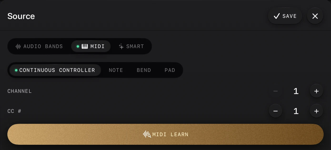
- Verify that your external hardware controllers are sending the correct signals at /tools/midi-tester. Check CC values, note velocities, and channel assignments.
- Download high quality, royalty free video content to test your reactive mappings at /loops. These clips provide distinct visual elements that react well to heavy parameter modulation.
What to do next
Once you understand the architecture of the audio pipeline and have secured a clean signal chain, you must integrate these concepts into your performance setup. Follow these precise steps to calibrate your rig for an upcoming show.
- Connect your audio interface to your DJ mixer via the Record Out ports and verify the input level in your system preferences.
- Load a reference track with a heavy kick drum and clear hi-hats. Route this track through the mixer into the interface.
- Open the visualizer and observe the incoming spectrum. Adjust the hardware input gain on your interface until the peak signals hit just below the maximum threshold.
- Set the noise gate to -60 dB to cut out electrical hum and floor noise.
- Map the bass band to the scale of a primary video layer. Tune the bass crossover frequency until only the kick drum triggers the scale effect.
- Map the high band to the opacity of an overlay layer. Tune the high crossover frequency until only the crisp cymbals trigger the flash.
- Test a transient extraction map by routing a transient trigger to a clip swap function. Verify that rapid drum fills cause rapid clip changes.
- Save this calibrated setup as your baseline template. Use this template as the starting point for every new venue you encounter.