Mapping audio frequencies and MIDI control data to visual parameters dictates exactly how your live visuals react to sound and physical input. A raw signal sent directly to a visual effect often looks chaotic. You must shape the data using modulation curves, minimum and maximum boundaries, and signal smoothing filters to create intentional, rhythmic visual changes. This technical guide explains the internal signal routing architecture in ImmerGround and shows you how to calibrate incoming control data for precise visual performance.
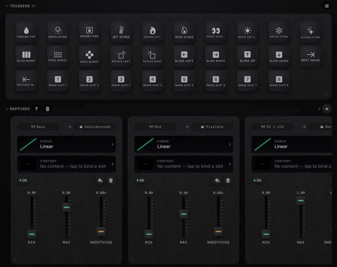
The Modulation Mapping System Architecture
The modulation mapping system operates as a massive routing matrix between incoming control signals and outgoing visual render parameters. Every frame, the engine reads the state of all audio inputs and MIDI controllers, normalizes the data to a standard floating point range, applies mathematical transformations, and updates the parameters of the active visual filters.
A mapping consists of three core components: a source, a destination, and a shape path. The source represents the origin of the control signal.
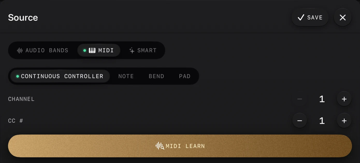
This can be a specific frequency band from the live microphone input, a frequency band from a local audio file, or a Continuous Control message from an external MIDI controller. The destination represents the target visual parameter.
This can be the rotation angle of a kaleidoscope, the block size of a pixelation effect, or the zoom scale of a source video. The shape path sits between the source and the destination.
It modifies the raw numerical value before the system hands it over to the rendering engine. When you create a new mapping, you instruct the engine to constantly monitor a specific input channel.
For audio sources, the engine performs a Fast Fourier shape on the incoming waveform. It splits the audible spectrum into distinct bands, measures the amplitude of each band, and converts that amplitude into a decimal value between zero and one.
For MIDI sources, the engine listens for the designated CC number on the specified MIDI channel. It takes the standard 7 bit integer value, ranging from zero to 127, and divides it by 127 to create a normalized decimal value between zero and one.
By normalizing all incoming signals to a zero to one range, the system allows you to hot swap sources without reconfiguring the entire shape path. You can map an audio bass band to a zoom effect for the first half of a show.
Then, you can delete that mapping and map a MIDI fader to the exact same zoom effect. The visual engine receives the same numerical format in both cases.
The system architecture guarantees a tight sync between the audio buffer, the MIDI event queue, and the screen refresh rate. The engine samples the control sources immediately before beginning the render pass for the current frame.
This eliminates frame lag and ensures the visuals stay locked to the rhythm of the music.
| Signal Source | Raw Data Format | Normalized Range | Typical Update Rate |
|---|---|---|---|
| Microphone Input | Float Array (FFT) | 0.0 to 1.0 | 60 frames per second |
| Local Audio File | Float Array (FFT) | 0.0 to 1.0 | 60 frames per second |
| MIDI CC Knob | 7-bit Integer (0-127) | 0.0 to 1.0 | Hardware dependent |
| MIDI CC Fader | 7-bit Integer (0-127) | 0.0 to 1.0 | Hardware dependent |
Understanding this normalized data flow is mandatory for mastering the rest of the mapping controls. Every curve, range slider, and smoothing filter operates on this zero to one decimal scale.
The numbers only translate into actual effect values at the very end of the signal chain.
Modulation Curves: Linear, Exponential, Logarithmic and S-Curve
A normalized control signal increases at a steady, constant rate from zero to one. If you route this linear signal directly to a visual parameter, the visual change will also happen at a steady, constant rate.
This linear behavior works well for basic fading tasks. However, it rarely produces musically pleasing results for sharp transients or deep filter sweeps.
Modulation curves allow you to alter the mathematical response of the signal path. They warp the zero to one scale to create faster or slower changes at different points in the movement.
The linear curve requires no mathematical transformation. A 50 percent input equals a 50 percent output.
You use the linear curve for MIDI faders that control master opacity or crossfaders between two clips. You want the physical position of the fader to perfectly match the visual state on the screen.
The exponential curve creates a slow initial rise that rapidly accelerates as it approaches the maximum value. This curve maps perfectly to parameters that require extreme precision at low values but rapid change at high values.
If you map a MIDI knob to a distortion effect using an exponential curve, turning the knob slightly from the zero position will produce very subtle changes. The distortion will remain controllable.
As you turn the knob past the halfway point, the effect will increase dramatically, allowing for intense, chaotic peaks. The exponential curve also works exceptionally well for audio mapping.
It acts like a noise gate. Low level background noise produces almost no visual output, while loud drum hits push the signal into the fast rising section of the curve, triggering massive visual bursts.
The logarithmic curve does the exact opposite of the exponential curve. It creates a rapid initial rise that slows down as it approaches the maximum value.
You use a logarithmic curve when you want a visual effect to snap to a high value immediately upon receiving input, but you want to fine tune the extreme upper limits. This curve works beautifully for mapping audio transients to scale parameters.
A snare drum hit will instantly trigger a massive zoom effect, but the tail of the audio signal will decay slowly, creating a lingering, elastic visual release. The S-Curve, or sigmoid curve, combines a slow start, a rapid middle section, and a slow end.
It creates smooth transitions between two distinct states. You use the S-Curve to prevent harsh, robotic movements.
If you map a MIDI button to a color inversion effect, a linear curve would create a hard flash. An S-Curve will ramp the color shift smoothly, creating a polished, professional look.
This curve excels at controlling parameters like blur radius or color saturation, where linear changes often feel rigid and mechanical.
| Curve Type | Mathematical Behavior | Best Audio Use Case | Best MIDI Use Case |
|---|---|---|---|
| Linear | Direct 1:1 translation | Ambient volume tracking | Opacity faders, crossfaders |
| Exponential | Slow start, fast finish | Snare hits, isolating loud peaks | Distortion knobs, glitch thresholds |
| Logarithmic | Fast start, slow finish | Bass drums, sustaining visual impact | Filter sweeps, rapid zoom hits |
| S-Curve | Slow start, fast middle, slow finish | Vocal volume tracking | Smooth color transitions, blur amounts |
You can swap curves on the fly while a mapping remains active. This allows you to audition different mathematical responses during a soundcheck and choose the curve that fits the acoustic profile of the room.
Setting Minimum and Maximum Parameter Bounds
Modulation curves shape the speed of the control signal, but minimum and maximum parameter bounds dictate the total range of motion. Without boundary limits, a control signal will always drive a visual parameter from its absolute lowest possible value to its absolute highest possible value.
For many effects, pushing a parameter to its absolute maximum will completely destroy the image, turning the screen into a mess of chaotic pixels. Parameter bounds allow you to constrain the effect to a usable, aesthetically pleasing range.
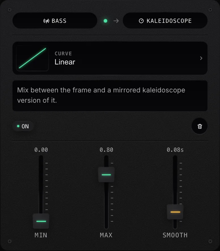
The minimum bound sets the resting state of the effect when the control signal sits at zero. The maximum bound sets the peak state of the effect when the control signal hits one.
By adjusting these two sliders on the mapping card, you define a specific window of operation for the visual parameter. Consider mapping the bass frequency band to a kaleidoscope rotation effect.
If you leave the bounds at their default zero and one positions, the screen will remain perfectly still during quiet moments. When a massive bass drop hits, the image will spin wildly out of control, making it impossible for the audience to see the original video clip.
2. Now, during a loud bass hit, the image will only rotate slightly, creating a tight, rhythmic twitch instead of a chaotic spin.
You retain the energetic response to the music, but you maintain the structural integrity of the visual composition. You can also use minimum and maximum bounds to invert the behavior of an effect.
By setting the minimum bound higher than the maximum bound, you force the visual parameter to move backwards as the control signal increases. This technique opens up entirely new creative possibilities.
You can map a MIDI fader to control the brightness of a clip. 0, pushing the fader up will actually make the clip darker.
This inverse mapping allows you to build complex control layouts where moving a single fader brightens one layer while simultaneously darkening another layer. Setting proper bounds requires constant testing and observation.
Every video clip reacts differently to visual effects. A high contrast geometric clip might withstand extreme pixelation, while a soft, organic clip might become unrecognizable with even a small amount of pixel distortion.
You must use the preview monitors to carefully calibrate the boundaries for every mapping in your project.
- Resting state definition: The minimum slider dictates exactly what the effect looks like when no audio plays and no MIDI knobs turn.
- Peak intensity limitation: The maximum slider prevents extreme control signals from breaking the visual engine or disorienting the crowd.
- Inverted motion: Crossing the minimum and maximum values reverses the mathematical logic, turning positive control signals into negative parameter changes.
- Narrow band mapping: Setting the minimum to 0.4 and the maximum to 0.6 confines the entire range of motion to a tiny, precise window for subtle texture shifts.
The bounds system operates after the modulation curve in the signal chain. The engine first applies the logarithmic or exponential math to the zero to one scale.
Then, it maps that warped scale onto your custom minimum and maximum boundaries. This combination of curves and limits provides total authority over the final visual output.
Signal Response Smoothing Filters
Live audio inputs and physical MIDI controllers generate messy data. A bass drum hit does not produce a perfect square wave.
It produces a complex cluster of frequencies that jitter rapidly. A human hand turning a MIDI knob does not move at a perfectly constant speed.
It hesitates, accelerates, and micro stutters. If you map these raw signals directly to visual parameters, the screen will strobe, flicker, and shake in an unpleasant manner.
Signal response smoothing filters eliminate this jitter and create fluid, continuous visual motion. Smoothing acts like an elastic band attached to the control signal.
Instead of instantly jumping to a new value, the visual parameter chases the control signal over time. The smoothing fader on the mapping card dictates the length of this chase time, measured in milliseconds.
A higher smoothing value creates a lazier, more fluid response. A lower smoothing value creates a tighter, more immediate response.
When mapping audio frequencies, smoothing is critical for removing high frequency noise from the signal path. If you map the mid frequency band to a color shift effect without any smoothing, the colors will strobe violently, potentially causing discomfort for the audience.
By increasing the smoothing value, you instruct the engine to average out the rapid fluctuations in the audio amplitude. The color shift will now glide gracefully in response to the overall volume envelope of the track, rather than reacting to every single microscopic transient.
Smoothing also plays a crucial role in MIDI control. Standard MIDI CC messages only provide 128 discrete steps of resolution.
If you map a MIDI knob to a slow pan effect, you will visibly see the image jump from pixel to pixel as you turn the knob. The visual motion will look stair stepped and digital.
Adding a small amount of smoothing forces the engine to interpolate the missing data between the 128 MIDI steps. The pan effect will glide smoothly across the screen, masking the low resolution limitations of the MIDI protocol.
| Signal Problem | Required Smoothing Strategy | Recommended Smoothing Range |
|---|---|---|
| Audio jitter / strobing visuals | Heavy smoothing to average the amplitude envelope | 150ms to 300ms |
| Stair-stepped MIDI knob movement | Light smoothing to interpolate between the 128 discrete data steps | 30ms to 60ms |
| Harsh transients breaking the composition | Moderate smoothing to round off the initial attack peak | 80ms to 120ms |
| Fast rhythmic sync required | Minimal smoothing to preserve the tight timing of the hit | 0ms to 20ms |
You must balance the desire for smooth visuals against the need for rhythmic accuracy. If you apply too much smoothing to an audio mapping, the visual effect will lag behind the beat of the music.
The audience will perceive a disconnect between the sound they hear and the images they see. You must tune the smoothing slider carefully to remove the jitter while maintaining a tight visual sync with the transient attacks.
Different musical genres require different smoothing approaches. A fast techno track with sharp, staccato drums demands very low smoothing values to keep the visuals punching on the grid.
A slow, ambient drone track benefits from extremely high smoothing values, allowing the visual parameters to drift lazily across the screen like clouds. The smoothing parameter is just as important as the source routing and the curve selection when building a dynamic visual performance.
Mapping Sound Bands vs MIDI Control Signals
You have two distinct methods for driving visual parameters: automated audio mapping and manual MIDI mapping. A professional visual setup utilizes both methods simultaneously to create a layered, complex performance.
Understanding the strengths and weaknesses of each signal type allows you to assign the correct tool to the correct visual task. Audio mapping excels at speed, accuracy, and automation.
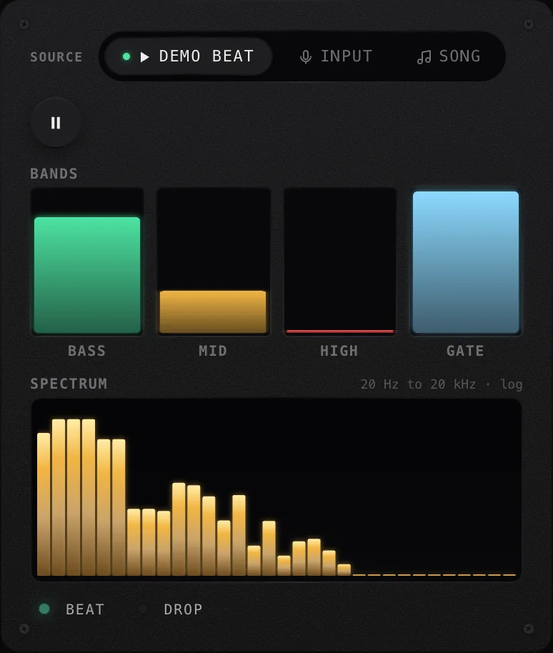
The engine analyzes the incoming sound in real time, reacting to frequency changes and volume spikes faster than humanly possible. You map audio bands to fast, rhythmic visual effects.
Bass frequencies trigger scale jumps and heavy distortion. Mid frequencies trigger color inversions and pixelation block sizes.
High frequencies trigger subtle noise layers and brightness flashes. Audio mapping handles the kinetic energy of the show, keeping the visuals locked to the tempo without requiring constant physical intervention.
However, audio mapping lacks structural intent. The system does not know if the current song is the climax of the set or a quiet breakdown.
It simply reacts to the numbers in the FFT array. If the music stops, the audio driven effects stop.
You cannot build long, slow tension using only sound analysis. MIDI control signals provide the structural intent that audio mapping lacks.
You use physical knobs, faders, and buttons to shape the overall narrative arc of the visual performance. You map MIDI faders to the master opacity of different video layers, allowing you to manually blend clips together.
You map MIDI knobs to the minimum and maximum bounds of the audio mappings, allowing you to manually increase or decrease the intensity of the audio reactive effects over time. You map MIDI buttons to route specific video clips to the screen, controlling the thematic content of the show.
- Bass Frequency Tracking: Use for heavy, structural changes like zoom, rotation, and high contrast thresholds.
- Mid Frequency Tracking: Use for textural changes like blur, pixelation, and chromatic aberration.
- MIDI Faders: Use for slow, deliberate actions like layer mixing, master brightness, and crossfading.
- MIDI Knobs: Use for fine tuning parameters like effect bounds, smoothing times, and color hue selection.
- MIDI Buttons: Use for immediate binary actions like clip triggering, strobe firing, and effect bypassing.
To connect external hardware, you will need a robust physical setup. If you run the engine on a Mac, you can connect class compliant MIDI controllers directly to the USB ports.
The operating system will recognize the hardware, and the application will immediately receive the CC data. If you run the engine on an iPad or an iPhone, you must use a powered USB-C hub.
The hub provides the necessary data connection to the device while simultaneously charging the battery. You must ensure your MIDI controller draws minimal power or use a controller with an independent power supply to prevent draining the battery of the mobile device during a long set.
The most effective performances combine both control paradigms. You might map the bass frequency to the scale of a 3D geometry clip, making the object pulse with the kick drum.
Simultaneously, you map a MIDI knob to the rotation axis of that same geometry. The audio provides the fast rhythmic pulse, while your hand provides the slow, evolving rotation.
The combination creates a visual output that feels both mathematically precise and uniquely human.
Advanced Multi-Mapping Strategies
The true potential of the modulation architecture reveals itself when you assign a single control source to multiple visual destinations simultaneously. A one to one mapping produces predictable results.
A one to many mapping produces complex, emergent visual behaviors that impossible to achieve with a single effect. Consider a scenario where you want a massive visual impact on every downbeat.
Mapping the kick drum to a simple zoom effect works, but it feels flat. Instead, you map the bass frequency band to three separate parameters simultaneously: the zoom scale, the red color channel intensity, and the blur radius.
Now, when the kick drum hits, the image scales up, flashes red, and blurs slightly at the edges. As the sound decays, the image shrinks, returns to its original color, and sharpens back into focus.
You have built a custom, composite visual effect driven by a single audio source. To execute this multi mapping strategy successfully, you must use different curves and bounds for each destination.
If you assign the exact same linear curve and zero to one bounds to all three parameters, the visual changes will overlap completely, often resulting in a messy, muddy image. You must separate the mathematical responses.
For the zoom scale, you use a logarithmic curve. This ensures the image jumps outward instantly with the initial transient of the kick drum.
5. This ensures the color shift ramps smoothly and does not completely overpower the original hues of the video clip.
For the blur radius, you use an exponential curve. This ensures the blur only triggers at the absolute peak volume of the audio signal, keeping the image sharp during quieter sections of the track.
You can also use inverse mapping bounds to create push and pull dynamics within a multi mapping setup. Map a MIDI knob to control both a pixelate effect and a kaleidoscope effect.
Set the pixelate bounds from zero to one. Set the kaleidoscope bounds from one to zero.
When the knob sits at the far left position, the screen shows a heavily fragmented kaleidoscope pattern. As you turn the knob to the right, the kaleidoscope structure slowly resolves back into a normal image, while the pixelation effect simultaneously increases, destroying the image in a completely different way.
The single knob crossfades between two distinct states of visual destruction.
| Control Source | Destination 1 (Curve / Bounds) | Destination 2 (Curve / Bounds) | Resulting Visual Behavior |
|---|---|---|---|
| Audio Bass Band | Zoom Scale (Logarithmic / 0 to 0.8) | Vignette Falloff (Exponential / 0 to 0.5) | Image pulses outward instantly, screen edges darken only on massive volume peaks. |
| Audio Mid Band | Color Hue (Linear / 0 to 1.0) | Saturation (Linear / 1.0 to 0.0) | Colors cycle rapidly with the sound, but extreme volume drops the saturation to black and white. |
| MIDI Mod Wheel | Blur Radius (S-Curve / 0 to 0.6) | Contrast (Linear / 0 to 0.8) | Pushing the wheel blurs the image smoothly while pushing the dark tones to pure black. |
Multi mapping requires extensive experimentation. You must constantly monitor the frame rate when stacking multiple heavy rendering effects on a single control source.
The engine handles complex routing matrices efficiently, but activating too many shader intensive effects simultaneously will eventually tax the graphics processing unit. Monitor the performance meters and disable unnecessary mappings to maintain a solid 60 frames per second output.
By mastering curves, bounds, smoothing, and multi mapping techniques, you move beyond basic visual playback. You construct an intelligent, reactive rendering system that interprets audio and physical input to generate a unique visual experience every time you perform.
Where to get free visual tools
Before purchasing hardware controllers or committing to a complex live setup, you can test these mapping concepts using our suite of browser based utilities. These tools run locally in your web browser and allow you to experiment with modulation routing, audio analysis, and MIDI data visualization.
- The Free Visualizer: Open the visualizer application in your browser. This tool includes the exact same mapping card interface detailed in this guide. You can route your microphone input to various effects, adjust the curves, set the minimum and maximum boundaries, and dial in the smoothing filters to see exactly how the math affects the visual output.
- Tempo Analysis: Use the BPM finder to analyze your audio tracks. Understanding the precise tempo of your music helps you calculate exact delay times and set up rhythmic MIDI trigger loops that stay perfectly in sync with the beat.
- Hardware Debugging: Connect your controller and open the MIDI tester. This diagnostic tool displays the exact raw data streaming from your hardware. You can verify that your knobs send full 0 to 127 resolution signals, check for jittery faders, and ensure your device sends data on the correct MIDI channel before mapping it to the visual engine.
- Content Library: Download high quality video clips from the loops library. We optimize all files in this directory for real time rendering and heavy effect modulation. They provide clean, high contrast starting points for testing your custom mapping logic.
What to do next
You now understand the mathematical foundation of audio and MIDI modulation. To translate this theory into a reliable live performance setup, you must implement these concepts methodically.
Follow these steps to build your custom mapping architecture.
- Connect your MIDI controller via USB and verify the signal flow using the testing tool linked above. Note the specific CC numbers assigned to your primary knobs and faders.
- Load a simple, high contrast geometric video loop into the engine to serve as a visual baseline. Do not start with complex, narrative video files.
- Create a single mapping from the audio bass band to a zoom or scale effect. Set the curve to logarithmic and lower the maximum bound to 0.3.
- Play a loud, percussive track and adjust the smoothing slider until the zoom effect pulses tightly with the kick drum without flickering.
- Create a second mapping from a MIDI knob to a blur or pixelate effect. Set the curve to linear and leave the bounds at zero and one.
- Practice manipulating the MIDI knob slowly while the audio mapping handles the fast rhythmic pulsing. Observe how the two control signals interact on the screen.
- Begin building multi mappings. Assign one MIDI fader to control the opacity of layer one, and assign that exact same MIDI fader, using inverted minimum and maximum bounds, to control the opacity of layer two. Practice crossfading between clips with a single physical movement.
- Save your project configuration. The engine stores all curves, bounds, smoothing times, and routing assignments in the project file, allowing you to recall your complex multi mappings instantly at the venue.